sfarrow is a package for reading and writing Parquet and Feather files with sf objects using arrow in R.
Simple features are a popular format for representing spatial vector data using data.frames and a list-like geometry column, implemented in the R package sf. Apache Parquet files are an open-source, column-oriented data storage format (https://parquet.apache.org/) which enable efficient read/writing for large files. Parquet files are becoming popular across programming languages and can be used in R using the package arrow.
The sfarrow implementation translates simple feature data objects using well-known binary (WKB) format for geometries and reads/writes Parquet/Feather files. A key goal of the package is for interoperability of the files (particularly with Python GeoPandas), so coordinate reference system information is maintained in a standard metadata format (https://github.com/geopandas/geo-arrow-spec). Note to users: this metadata format is not yet stable for production uses and may change in the future.
Installation
sfarrow is available through CRAN with:
install.packages('sfarrow')or it can be installed from Github with:
devtools::install_github("wcjochem/sfarrow@main")Load the library to begin using it.
arrow package
The installation requires the Arrow library which should be installed with the R package arrow dependency. However, some systems may need to follow additional steps to enable full support of that library. Please refer to the arrow documentation.
Basic usage
Reading Parquet data of spatial files created with Python GeoPandas.
# load Natural Earth low-res dataset.
# Created in Python with geopandas.to_parquet()
path <- system.file("extdata", "world.parquet", package = "sfarrow")

world <- st_read_parquet(path)

world
#> Simple feature collection with 177 features and 5 fields
#> Geometry type: GEOMETRY
#> Dimension:     XY
#> Bounding box:  xmin: -180 ymin: -90 xmax: 180 ymax: 83.64513
#> Geodetic CRS:  WGS 84
#> First 10 features:
#>      pop_est     continent                     name iso_a3 gdp_md_est
#> 1     920938       Oceania                     Fiji    FJI  8.374e+03
#> 2   53950935        Africa                 Tanzania    TZA  1.506e+05
#> 3     603253        Africa                W. Sahara    ESH  9.065e+02
#> 4   35623680 North America                   Canada    CAN  1.674e+06
#> 5  326625791 North America United States of America    USA  1.856e+07
#> 6   18556698          Asia               Kazakhstan    KAZ  4.607e+05
#> 7   29748859          Asia               Uzbekistan    UZB  2.023e+05
#> 8    6909701       Oceania         Papua New Guinea    PNG  2.802e+04
#> 9  260580739          Asia                Indonesia    IDN  3.028e+06
#> 10  44293293 South America                Argentina    ARG  8.794e+05
#>                          geometry
#> 1  MULTIPOLYGON (((180 -16.067...
#> 2  POLYGON ((33.90371 -0.95, 3...
#> 3  POLYGON ((-8.66559 27.65643...
#> 4  MULTIPOLYGON (((-122.84 49,...
#> 5  MULTIPOLYGON (((-122.84 49,...
#> 6  POLYGON ((87.35997 49.21498...
#> 7  POLYGON ((55.96819 41.30864...
#> 8  MULTIPOLYGON (((141.0002 -2...
#> 9  MULTIPOLYGON (((141.0002 -2...
#> 10 MULTIPOLYGON (((-68.63401 -...
plot(sf::st_geometry(world))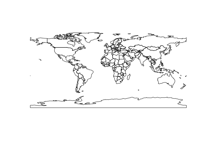
Writing sf objects to Parquet format files. These Parquet files created with sfarrow can be read within Python using GeoPandas.
nc <- sf::st_read(system.file("shape/nc.shp", package="sf"), quiet=TRUE)

st_write_parquet(obj=nc, dsn=file.path(tempdir(), "nc.parquet"))
#> Warning: This is an initial implementation of Parquet/Feather file support and
#> geo metadata. This is tracking version 0.1.0 of the metadata
#> (https://github.com/geopandas/geo-arrow-spec). This metadata
#> specification may change and does not yet make stability promises.  We
#> do not yet recommend using this in a production setting unless you are
#> able to rewrite your Parquet/Feather files.

# read back into R
nc_p <- st_read_parquet(file.path(tempdir(), "nc.parquet"))

nc_p
#> Simple feature collection with 100 features and 14 fields
#> Geometry type: MULTIPOLYGON
#> Dimension:     XY
#> Bounding box:  xmin: -84.32385 ymin: 33.88199 xmax: -75.45698 ymax: 36.58965
#> Geodetic CRS:  NAD27
#> First 10 features:
#>     AREA PERIMETER CNTY_ CNTY_ID        NAME  FIPS FIPSNO CRESS_ID BIR74 SID74
#> 1  0.114     1.442  1825    1825        Ashe 37009  37009        5  1091     1
#> 2  0.061     1.231  1827    1827   Alleghany 37005  37005        3   487     0
#> 3  0.143     1.630  1828    1828       Surry 37171  37171       86  3188     5
#> 4  0.070     2.968  1831    1831   Currituck 37053  37053       27   508     1
#> 5  0.153     2.206  1832    1832 Northampton 37131  37131       66  1421     9
#> 6  0.097     1.670  1833    1833    Hertford 37091  37091       46  1452     7
#> 7  0.062     1.547  1834    1834      Camden 37029  37029       15   286     0
#> 8  0.091     1.284  1835    1835       Gates 37073  37073       37   420     0
#> 9  0.118     1.421  1836    1836      Warren 37185  37185       93   968     4
#> 10 0.124     1.428  1837    1837      Stokes 37169  37169       85  1612     1
#>    NWBIR74 BIR79 SID79 NWBIR79                       geometry
#> 1       10  1364     0      19 MULTIPOLYGON (((-81.47276 3...
#> 2       10   542     3      12 MULTIPOLYGON (((-81.23989 3...
#> 3      208  3616     6     260 MULTIPOLYGON (((-80.45634 3...
#> 4      123   830     2     145 MULTIPOLYGON (((-76.00897 3...
#> 5     1066  1606     3    1197 MULTIPOLYGON (((-77.21767 3...
#> 6      954  1838     5    1237 MULTIPOLYGON (((-76.74506 3...
#> 7      115   350     2     139 MULTIPOLYGON (((-76.00897 3...
#> 8      254   594     2     371 MULTIPOLYGON (((-76.56251 3...
#> 9      748  1190     2     844 MULTIPOLYGON (((-78.30876 3...
#> 10     160  2038     5     176 MULTIPOLYGON (((-80.02567 3...
plot(sf::st_geometry(nc_p))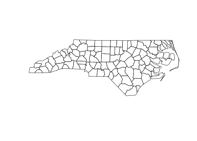
For additional examples please see the vignettes.